Graph algorithms
Introduction
The graph is a mathematical structure used to describe a set of objects in which
some pairs of objects are "related" in some sense. Generally, we consider
those objects as abstractions named nodes (also called vertices).
Aforementioned relations between nodes are modelled by an abstraction named
edge (also called relationship).
It turns out that a lot of real-world problems can be successfully modeled using graphs. Some natural examples would contain railway networks between cities, computer networks, piping systems and Memgraph itself.
This article outlines some of the most important graph algorithms that are internally used by Memgraph. We believe that advanced users could significantly benefit from obtaining basic knowledge about those algorithms. The users should also note that this article does not contain an in-depth analysis of algorithms and their implementation details since those are well documented in the appropriate literature and, in our opinion, go well out of scope for user documentation. That being said, we will include the relevant information for using Memgraph effectively and efficiently.
Contents of this article include:
Breadth First Search
Breadth First Search is a way of traversing a graph data structure. The traversal starts from a single node (usually referred to as source node) and, during the traversal, breadth is prioritized over depth, hence the name of the algorithm. More precisely, when we visit some node, we can safely assume that we have already visited all nodes that are fewer edges away from a source node. An interesting side-effect of traversing a graph in BFS order is the fact that, when we visit a particular node, we can easily find a path from the source node to the newly visited node with the least number of edges. Since in this context we disregard the edge weights, we can say that BFS is a solution to an unweighted shortest path problem.
The algorithm itself proceeds as follows:
- Keep around a set of nodes that are equidistant from the source node. Initially, this set contains only the source node.
- Expand to all not yet visited nodes that are a single edge away from that set. Note that the set of those nodes is also equidistant from the source node.
- Replace the set with a set of nodes obtained in the previous step.
- Terminate the algorithm when the set is empty.
The order of visited nodes is nicely visualized in the following animation from Wikipedia. Note that each row contains nodes that are equidistant from the source and thus represents one of the sets mentioned above.
The standard BFS implementation skews from the above description by relying on
a FIFO (first in, first out) queue data structure. Nevertheless, the
functionality is equivalent and its runtime is bounded by O(|V| + |E|) where
V denotes the set of nodes and E denotes the set of edges. Therefore,
it provides a more efficient way of finding unweighted shortest paths than
running Dijkstra's algorithm on a graph
with edge weights equal to 1.
Weighted Shortest Path
In graph theory, weighted shortest path problem is the problem of finding a path between two nodes in a graph such that the sum of the weights of edges connecting nodes on the path is minimized.
Dijkstra's algorithm
One of the most important algorithms for finding weighted shortest paths is Dijkstra's algorithm. Our implementation uses a modified version of this algorithm that can handle length restriction. The length restriction parameter is optional and when it's not set it could increase the complexity of the algorithm. It is important to note that the term "length" in this context denotes the number of traversed edges and not the sum of their weights.
The algorithm itself is based on a couple of greedy observations and could be expressed in natural language as follows:
- Keep around a set of already visited nodes along with their corresponding
shortest paths from source node. Initially, this set contains only the
source node with the shortest distance of
0. - Find an edge that goes from a visited node to an unvisited one such that the shortest path from source to the visited node increased by the weight of that edge is minimized. Traverse that edge and add a newly visited node with appropriate distance to the set of already visited nodes.
- Repeat the process until the destination node is visited.
The described algorithm is nicely visualized in the following animation from Wikipedia. Note that edge weights correspond to the Euclidean distance between nodes which represent points on a plane.
Using appropriate data structures the worst-case performance of our
implementation can be expressed as O(|E| + |V|log|V|) where E denotes
the set of edges and V denotes the set of nodes.
A sample query that finds a shortest path between two nodes looks as follows:
MATCH (a {id: 723})-[edge_list *wShortest 10 (e, n | e.weight) total_weight]-(b {id: 882}) RETURN *;
This query has an upper bound length restriction set to 10. This means that no
path that traverses more than 10 edges will be considered as a valid result.
Upper Bound Implications
Since the upper bound parameter is optional, we can have different results based on this parameter.
Consider the following graph and sample queries.
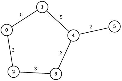
MATCH (a {id: 0})-[edge_list *wShortest 3 (e, n | e.weight) total_weight]-(b {id: 5}) RETURN *;
MATCH (a {id: 0})-[edge_list *wShortest (e, n | e.weight) total_weight]-(b {id: 5}) RETURN *;
The first query will try to find the weighted shortest path between nodes 0
and 5 with the restriction on the path length set to 3, and the second query
will try to find the weighted shortest path with no restriction on the path
length.
The expected result for the first query is 0 -> 1 -> 4 -> 5 with the total
cost of 12, while the expected result for the second query is
0 -> 2 -> 3 -> 4 -> 5 with the total cost of 11. Obviously, the second
query can find the true shortest path because it has no restrictions on the
length.
To handle cases when the length restriction is set, weighted shortest path algorithm uses both node and distance as the state. This causes the search space to increase by the factor of the given upper bound. On the other hand, not setting the upper bound parameter, the search space might contain the whole graph.
Because of this, one should always try to narrow down the upper bound limit to be as precise as possible in order to have a more performant query.
Where to next?
For some real-world application of WSP we encourage you to visit our article Exploring the European road network which was specially crafted to showcase our graph algorithms.