How to use built-in query modules
Memgraph Community edition comes with a set of Python query modules based on
the NetworkX library of algorithms. The modules
are already packaged within all Memgraph packages, but NetworkX might have to
be installed by running the following command:
pip3 install networkx
info
NOTE: The following "How to Guides" provide an explanation of basic usage. To find
out more details about each module and documentation of each procedure, please
take a look at our Reference guide
or the query module source files. The files are located in the directory
/usr/lib/memgraph/query_modules.
NetworkX Algorithms Module
In addition to standalone community graph algorithms implemented as Python
modules, we implemented a module providing NetworkX integration with Memgraph.
This module, named nxalgo, provides a comprehensive set of thin wrappers
around most of the algorithms present in the NetworkX package. The wrapper
functions now have the capability to create a NetworkX compatible graph-like
object that can stream the native database graph directly, saving
on memory usage significantly.
For example, you can run the Page Rank algorithm on the data stored in Memgraph. To illustrate the functionality, the following graph will be used:
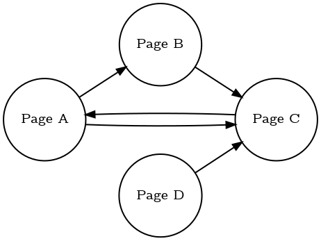
To load the graph into Memgraph, the following query should be used:
CREATE (na {name: "Page A"})
CREATE (nb {name: "Page B"})
CREATE (nc {name: "Page C"})
CREATE (nd {name: "Page D"})
CREATE (na)-[:e]->(nb)
CREATE (na)-[:e]->(nc)
CREATE (nc)-[:e]->(na)
CREATE (nb)-[:e]->(nc)
CREATE (nd)-[:e]->(nc);
By executing nxalg.pagerank(), Memgraph will return the rank for each
node as follows:
CALL nxalg.pagerank() YIELD *;
+--------------------+----------+
| node               | rank     |
+--------------------+----------+
| ({name: "Page C"}) | 0.39415  |
| ({name: "Page D"}) | 0.0375   |
| ({name: "Page A"}) | 0.372526 |
| ({name: "Page B"}) | 0.195824 |
+--------------------+----------+
NetworkX algorithms are located inside the nxalg.py file installed with
your Memgraph package in /usr/lib/memgraph/query_modules.
Graph Analyzer
The purpose of this module is to get more insights about the stored graph. To illustrate functionality the following graph will be used:
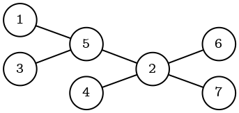
To create the graph, the following query should be executed:
CREATE (n1)
CREATE (n2)
CREATE (n3)
CREATE (n4)
CREATE (n5)
CREATE (n6)
CREATE (n7)
CREATE (n1)-[:e]->(n5)
CREATE (n3)-[:e]->(n5)
CREATE (n5)-[:e]->(n2)
CREATE (n4)-[:e]->(n2)
CREATE (n2)-[:e]->(n6)
CREATE (n2)-[:e]->(n7);
To analyze the whole graph, let's run the following query:
CALL graph_analyzer.analyze() YIELD *;
Results should be similar to the ones below.
+-------------------------------------------+-------------------------+
| name                                      | value                   |
+-------------------------------------------+-------------------------+
| "Number of nodes"                         | "7"                     |
| "Number of edges"                         | "6"                     |
| "Number of bridges"                       | "6"                     |
| "Number of articulation points"           | "2"                     |
| "Average degree"                          | "0.8571428571428571"    |
| "Sorted nodes degree"                     | "[(16, 4),(19, 3), ..." |
| "Self loops"                              | "0"                     |
| "Is bipartite"                            | "True"                  |
| "Is planar"                               | "True"                  |
| "Is biconnected"                          | "False"                 |
| "Is weakly connected"                     | "True"                  |
| "Number of weakly connected components"   | "1"                     |
| "Is strongly connected"                   | "False"                 |
| "Number of strongly connected components" | "7"                     |
| "Is DAG"                                  | "True"                  |
| "Is eulerian"                             | "False"                 |
| "Is forest"                               | "True"                  |
| "Is tree"                                 | "True"                  |
+-------------------------------------------+-------------------------+
To analyze a sub-graph, relevant nodes and edges have to be collected by
combining MATCH and WITH clauses. Once everything is collected,
analyze_subgraph procedure can be called as follows:
MATCH (n)-[e]->(m) WITH collect(n) as nodes, collect(e) as edges
CALL graph_analyzer.analyze_subgraph(nodes, edges) YIELD name, value
RETURN name, value;
Weakly Connected Components
The wcc.py query module can run
WCC analysis on
a sub-graph of the whole graph. To illustrate the number of weakly connected
components and nodes within each component, the following graph will be used:

To create the graph, run the following query:
CREATE (n1 {id: 1})
CREATE (n2 {id: 2})
CREATE (n3 {id: 3})
CREATE (n4 {id: 4})
CREATE (n1)-[:e]->(n2)
CREATE (n3)-[:e]->(n4);
The following query will do the calculation:
MATCH (n)-[e]->(m) WITH collect(n) as nodes, collect(e) as edges
CALL wcc.get_components(nodes, edges) YIELD components, n_components
RETURN components, n_components;
The expected result follows:
+--------------------------------------------------+--------------+
| components                                       | n_components |
+--------------------------------------------------+--------------+
| [[({id: 1}), ({id: 2})], [({id: 3}), ({id: 4})]] | 2            |
+--------------------------------------------------+--------------+
Please keep in mind that after the MATCH clause there can be a WHERE clause
with an arbitrary expression to further filter matched set of results.
Low-level optimized graph algorithms (Enterprise)
If you have purchased Memgraph's Enterprise edition, you have access to certain graph algorithms in the form of query modules. These modules were implemented by our own team using C++ and should offer some additional performance benefits. Currently, we have implemented the following algorithms:
- Louvain algorithm for community detection.
- Weakly connected components.
Louvain algorithm for community detection
In essence, this algorithm is a heuristic method which can be used to extract the community structure of fairly sizeable networks. In the simplest of terms, the algorithm attempts to assign graph nodes to communities in a way that maximizes the so-called modularity measure. For more details, we advise you to study the original paper.
This query module should be provided as a shared object (.so) file called
louvain.so. Assuming the standard installation on Debian, that file should be
located in /usr/lib/memgraph/query_modules. Again, we can simply run Memgraph with
the following command:
systemctl start memgraph
When using Docker, the equivalent would be the following:
docker run -p 7687:7687 \
  -v mg_lib:/var/lib/memgraph -v mg_log:/var/log/memgraph -v mg_etc:/etc/memgraph \
  memgraph
Suppose that Memgraph is currently storing a graph as depicted in the figure below where numbers in the vertices are stored as properties in the graph.
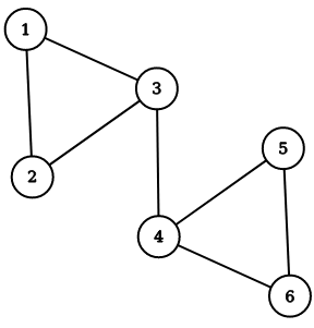
To create the above graph, execute the following query:
CREATE (n1 {number: 1})
CREATE (n2 {number: 2})
CREATE (n3 {number: 3})
CREATE (n4 {number: 4})
CREATE (n5 {number: 5})
CREATE (n6 {number: 6})
CREATE (n1)-[:e]->(n2)
CREATE (n1)-[:e]->(n3)
CREATE (n2)-[:e]->(n3)
CREATE (n3)-[:e]->(n4)
CREATE (n4)-[:e]->(n5)
CREATE (n4)-[:e]->(n6)
CREATE (n5)-[:e]->(n6);
Let's run the following query:
CALL louvain.communities() YIELD community, id;
We should get a result similar to:
+-----------+-----------+
| community | id        |
+-----------+-----------+
| 1         | 5         |
| 1         | 4         |
| 1         | 3         |
| 0         | 2         |
| 0         | 0         |
| 0         | 1         |
+-----------+-----------+
The procedure returns mappings from internal node IDs to communities. In order to return the nodes instead of the IDs you should execute the following query:
CALL louvain.communities() YIELD community, id MATCH (n) WHERE ID(n) = id RETURN community, n;
We should observe the following result:
+---------------+---------------+
| community     | n             |
+---------------+---------------+
| 1             | ({number: 6}) |
| 1             | ({number: 5}) |
| 1             | ({number: 4}) |
| 0             | ({number: 3}) |
| 0             | ({number: 1}) |
| 0             | ({number: 2}) |
+---------------+---------------+
As you can see, vertices numbered 1, 2 and 3 belong to one community, while vertices numbered 4, 5 and 6 belong to another community.
If you wish to know the exact graph modularity after running Louvain, you can run the following query:
CALL louvain.modularity() YIELD modularity;
In our example, the result should be:
+------------+
| modularity |
+------------+
| 0.357143   |
+------------+
If you wish, you can model the "strength of connection" between two nodes by
specifying the weight of that edge. To do that, you need to add a property on
that edge named weight which stores a real value. Naturally, larger weights
correspond to stronger connections. If you don't explicitly specify the weight
of a certain edge, its weight will internally default to 1. It's also
important to note that weights are internally represented as 64-bit floating
point numbers.
Finally, we should also state that the runtime of this algorithm (assuming we let it run until convergence) is not known. It merely appears to run in O(nlog(n)).
Weakly Connected Components
One of the most important features you might be interested in when exploring a certain graph is its connectivity. There are many ways in which we might express to which extent we are interested in the connectivity of a graph, but one of the simplest ones is by counting the number of its weakly connected components and by determining which vertex corresponds to which connected component.
The concept of weakly connected components is natural and simple, two nodes belong to the same component if a path between them exists in a given graph. Otherwise, we say those nodes are disconnected.
This query module should be provided as a shared object (.so) file called
connectivity.so. Assuming the standard installation on Debian, that file
should be located in /usr/lib/memgraph/query_modules. Again, we can simply run
Memgraph with the following command:
systemctl start memgraph
When using Docker, the equivalent would be the following:
docker run -p 7687:7687 \
  -v mg_lib:/var/lib/memgraph -v mg_log:/var/log/memgraph -v mg_etc:/etc/memgraph \
  memgraph
Suppose that Memgraph is currently storing a graph as depicted in the figure below where numbers in the vertices are stored as properties in the graph. This graph obviously has 4 weakly connected components.

To create the above graph, execute the following query:
CREATE (n1 {number: 1})
CREATE (n2 {number: 2})
CREATE (n3 {number: 3})
CREATE (n4 {number: 4})
CREATE (n5 {number: 5})
CREATE (n6 {number: 6})
CREATE (n7 {number: 7})
CREATE (n8 {number: 8})
CREATE (n9 {number: 9})
CREATE (n10 {number: 10})
CREATE (n11 {number: 11})
CREATE (n12 {number: 12})
CREATE (n13 {number: 13})
CREATE (n14 {number: 14})
CREATE (n15 {number: 15})
CREATE (n1)-[:e]->(n2)
CREATE (n1)-[:e]->(n3)
CREATE (n2)-[:e]->(n3)
CREATE (n5)-[:e]->(n6)
CREATE (n6)-[:e]->(n7)
CREATE (n6)-[:e]->(n8)
CREATE (n7)-[:e]->(n9)
CREATE (n7)-[:e]->(n10)
CREATE (n8)-[:e]->(n11)
CREATE (n12)-[:e]->(n13)
CREATE (n12)-[:e]->(n14)
CREATE (n12)-[:e]->(n15)
CREATE (n13)-[:e]->(n14)
CREATE (n13)-[:e]->(n15)
CREATE (n14)-[:e]->(n15);
Let's run the following query:
CALL connectivity.weak() YIELD component, id;
We should get a result similar to:
+-----------+-----------+
| component | id        |
+-----------+-----------+
| 3         | 14        |
| 3         | 13        |
| 3         | 12        |
| 3         | 11        |
| 2         | 10        |
| 2         | 9         |
| 2         | 8         |
| 2         | 7         |
| 2         | 6         |
| 0         | 1         |
| 0         | 0         |
| 0         | 2         |
| 1         | 3         |
| 2         | 4         |
| 2         | 5         |
+-----------+-----------+
The procedure returns mappings from internal node IDs to components. In order to return the nodes instead of the IDs you should execute the following query:
CALL connectivity.weak() YIELD component, id MATCH (n) WHERE ID(n) = id RETURN component, n;
We should observe the following result:
+----------------+----------------+
| component      | n              |
+----------------+----------------+
| 3              | ({number: 15}) |
| 3              | ({number: 14}) |
| 3              | ({number: 13}) |
| 3              | ({number: 12}) |
| 2              | ({number: 11}) |
| 2              | ({number: 10}) |
| 2              | ({number: 9})  |
| 2              | ({number: 8})  |
| 2              | ({number: 7})  |
| 0              | ({number: 2})  |
| 0              | ({number: 1})  |
| 0              | ({number: 3})  |
| 1              | ({number: 4})  |
| 2              | ({number: 5})  |
| 2              | ({number: 6})  |
+----------------+----------------+
As expected, nodes numbered 1, 2, and 3 are all in one connected component, node numbered 4 is in its own component, nodes numbered 5, 6, 7, 8, 9, 10, and 11 are in another component and, finally, nodes numbered 12, 13, 14 and 15 are in the last component.